What is it?
After replicating two models I respected, for this third and final model, I wanted to venture out into my own territory and try something completely new!
The origin story of this model will take a few minutes, so buckle up! I started this journey by exploring the concept of Expected Points Added (EPA). True to form, I recreated the implementation outlined in the original nflWAR paper[1]. I learned a lot diving into the minutiae, with the most important learning that EPA is a great tool for quantifying the value of the what happened on each play. It uses the average expectation of each play’s starting condition (field location, down, distance, etc.) to determine the relative value of the result of the play using a highly accurate calibration curve to infer the expected value of each play’s “state”.
My first attempt at a new model was instead of using the average expectation, only use each quarterback’s plays to determine their own expectation. But this was an abject disaster! To put it briefly, if you benchmark each quarterback by their own expectation, it will overvalue bad quarterbacks when they finally do something good and completely undervalue good quarterbacks. Not what we want!
The method I finally arrived at was instead of quantifying the result of the play, can we quantify the value of the play-calling decision? In other words, when the coach calls for a deep pass on 2nd and short, is that a valuable decision regardless of the outcome (and putting luck aside)? And does knowing which teams make optimum play calls provide us an information edge? These questions will form the basis of my Decision Rating Model.
Why is it Cool?
The EPA method is ubiquitous in NFL Analytics circles and is an excellent metric for measuring play value. My idea is that the EPA method does a good job of measuring what happened on a play but not if the decision was the correct one. Therefore, my model will leverage the excellent framework of EPA but focus it through a novel lens: quantifying play-calling decision-making.
The Model
Data Sources
This model requires play-by-play data (including EPA) for every game. Luckily, all this information is available through our handy-dandy nflfastR[2][3] source. Like our other two models, we’ll be considering the 2003 - 2023 seasons for performance evaluations, but training data will go back to 1999 for initial model training.
Setup
This model has a bit more under-the-hood than the other two models.
In the EPA method, the parameter listed in the Appendix are used as inputs into a XGBoost classifier to predict the probability of the next score (touchdown, field goal, safety, no score, opponent field goal, opponent touchdown, or opponent safety). By doing so, you can figure out the expected value of the position team before and after the play. That difference is the Expected Points Added of the play.
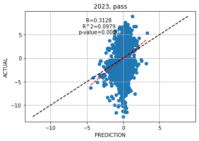
With the EPA for a play known, I trained a XGBoost regressor to predict the EPA (i.e., the result) of a play, given the same input parameters plus some pass or run-specific parameters (see Appendix). This was done with separate models for running and passing plays and therefore, I’ve naturally excluded special teams plays. Because play outcomes, and therefore EPA, are fundamentally unpredictable, I didn’t expect to get great results and you see that in the standard Bisector Plot below, shown for the 2023 passing plays. What’s more important is that there is some correlation between the prediction and EPA (R2 ~0.10) and I can therefore use the model to quantify the average outcome of each play given its initial state.
The regressor is trained on a season-by-season rolling basis, using all data for prior seasons. For example, the first season considered, 2003, is trained using data from 1999-2002 data. Once the regressor is trained and has been used to predict the EPA for each run and pass play, we sum up the Play-Calling Expectation (PCE) and EPA for each team’s running and passing plays for each game. For each team, these two metrics are averaged for all previous games in the season. Then, I compute the team’s Decision Rating as:
The parameters a and b were determined empirically to both be 0.5 as the value that optimized win prediction accuracy. Therefore, Decision Rating ends up being a equal-weighted blend between the team’s playing-calling decision quality and their results.
Finally, for each matchup, the predicted winner is the one with the higher Decision Rating, with the predicted spread being the difference between the teams’ Decision Ratings.
The Results
I’d like to visualize what this model is doing with a couple of examples from the 2023 season. Please note that the y-axis is in terms of rolling average expected points by a team’s offense, which is a differential measurement. In other words, positive values mean that the offense is outscoring the other team and a negative means the opposite.
First we have Green Bay, where you can see a well-coached but young team as they navigate their season:
Their PCE was very stable throughout the year, which shows that Head Coach Matt LaFleur had a consistent play-calling vision throughout the season.
They over-performed their PCE in the first two games of the season with a blowout win against the Bears and a solid offensive performance against Atlanta.
After that, the offense stagnated and under-performed their PCE as they faced tougher opponents and their young team struggled with growing pains
They turned things around mid-season with the big Thanksgiving Day win against Detroit. From that point on, their young offense found their footing and their AvgEPA converged with their PCE.
As a point of comparison is their divisional rival, the Detroit Lions. Again, we see a well-coached team but one that would appear to over-achieve offensively.
Their PCE was stable, and even slightly increasing throughout the year, which shows Dan Campbell and Ben Johnson’s steady & effective offensive gameplay.
Throughout the season, their offensive EPA was almost always greater than their EPA, indicating that they were over-achieving relative to the plays they were calling.
For this reasons, Detroit may be a candidate for offensive regression in the 2024 season.
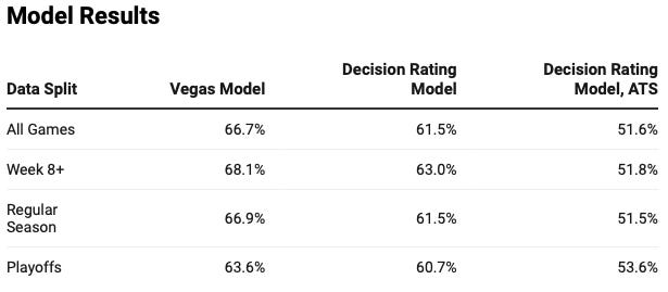
Moving to to how this model fairs in prediction tasks, I’ve computed the Win-Loss and Against the Spread (ATS) accuracies in the same fashion as the previous two models. The results are shown in the table below. The accuracy may be slightly less than the ~64% of the previous two models but I’m hoping the model is different enough to help us next time when we combine the three models in an ensemble voter.
The Final Dive
In this post, I leveraged my learnings from diving in the Expected Points Added methodology to create a new model, the Decision Rating Model. This model weights both a team’s average past success with its average past Play-Calling Expectation when evaluating a team’s value. We were able to see how PCE & EPA interact throughout the season for a couple of example teams. And then using this model for prediction tasks, we get modest results but ones that I hope are different enough from the previous models to be useful in an ensemble voting model.
The next post is going to dive into some really exciting topics on Condorcet’s Jury Theorem, Voting Models, and more, so I hope to see you there!
Appendix
EPA Model Inputs
Down
“Goal to Go” flag
Yardline
“Under two minutes in the half” flag
Seconds remaining in the half
log(Yards to Go for 1st down)
“Possession team is home team” flag
Home team’s score differential
Possession team timeouts remaining
Defending team timeouts remaining
Stadium roof type
Additional PCE Model Inputs for Pass Plays
Air yards
QB scramble flag
Pass play flag
“QB spiked the ball” flag
“Shotgun formation” flag
“No huddle play” flag
Route depth label
Pass location label
Additional PCE Model Inputs for Run Plays
QB scramble flag
“Shotgun formation” flag
“No huddle play” flag
Run type label
Run gap label
References
nflWAR: A Reproducible Method for Offensive Player Evaluation in Football, Yurko, Ventura, Horowitz.
https://fivethirtyeight.com/methodology/how-our-nfl-predictions-work/


Too much data stuff. You need to be like Dan Campbell and go with your gut! Damn the rules! Damn the stats! Neeeeeeerd! I was elected to lead, not to read.